dung counting
Introduction
The aim of this guide is to outline how a dung count can be used to estimate deer numbers. The Census Introduction guide should be regarded as companion reading, this guide also links to the Cull Planning guide.
General
Dung counts can indicate both the distribution and total number of deer in an area.
Dung counts:
- provide a means of estimating deer numbers in woodlands where visual counts may be difficult
- may be the most cost-effective means for measuring deer density in large areas of woodland
It should be noted that:
- Movement of deer in and out of an area may occur and, if significant, can produce highly misleading results unless the majority of the deer range is included or movements are predictable and the count timing takes account of that.
- It can be difficult to distinguish between the dung of different species. If confusion is likely it may be best not to try dung counting, or to treat all species as one and accept that the data will be of little use in cull planning for individual species, but could still be used as an index of overall deer activity.
- Because deer do not use their range in an even way and because dung decays at different rates in different habitats, it is necessary to “stratify” the deer range into habitat types and to carry out counts separately in each.
- This can significantly increase the amount of work to be done.
- There are many ways of arriving at estimates of deer numbers apart from dung counts. Wherever possible results from dung counts should be considered with results from other methods, each hopefully adding confidence to the other. For instance, although dung counts only estimate total numbers, some idea of sex and age class can be gained from visual census and applied to the dung count totals.
Dung counting is an “indirect” method of estimating deer numbers that avoids the difficulties of having to see deer to count them. The basic principle is that the more dung is present the more deer there must have been to produce it.
There are two complicating factors, dung persists for some time but the rate at which it decays (decay rate) is highly variable, secondly, the rate at which deer produce dung (defecation rate) although fairly constant, can vary.
The two main methods of dung counting attempt to take decay and defecation rate into account but there is always a degree of inaccuracy in results. One method is described here.
A recently developed third method combining FAR and FSC is described Bulletin 128 (see Further Info).
The method most widely recommended is the “faecal accumulation rate” (FAR) method described below.
| Method | description | pros | cons |
|---|---|---|---|
| Faecal Accumulation Rate (FAR) | Plots are marked out, dung is marked or removed. Dung is re-counted at return visit | Provided no dung has had time to decay, decay rate variable is removed from calculation. | Requires two visits |
| Faecal Standing Crop (FSC) | Plots are marked and dung counted. | Single visit required | Decay rate must be determined by multiple visits in each habitat type, for at least a 12 month period before the count. |
FAR method
Usually deer produce dung as loose pellets and deposit them periodically as “pellet groups” either in heaps or as a “string” of pellets if they are moving. A pellet group is any collection of six or more identifiable pellets produced at the same time. All dung counting techniques measure the amount of dung by counting the number of groups produced.
The FAR method is based on the principle that defecation rates are fairly constant within species. An area is visited and cleared of dung (or the dung is marked in some way). The site is then re-visited a known time later and the new dung counted. The number of deer that would have had to have been present to produce that amount of dung over the time period can then be calculated.
The method effectively counts “deer days”, that is it does not allow for the fact that the same amount of dung could be deposited either by deer present through the whole period in constant numbers, or by a larger herd that spent less time there.
Before the count
- Identify the size of the area to be surveyed, taking into account possible movement of deer.
- Break down the area into different habitats either by age, vegetation type or deer usage to allow samples to be stratified.
Examples of habitat stratification
Woodland habitat
Conifer/Broadleaved establishment 0-5 years old
Conifer/Broadleaved pre-thicket 5-10 years old
Conifer/Broadleaved pole stage or pre-felling
Mature forest/woodland
Coppice
Open habitat
Bare ground
Grass rides or glades
Moor or heath
Fields
- Prior to fieldwork, become familiar with the different species present using local knowledge, other signs, or by comparing found dung with known species dung.
- Choose a time of year when ground vegetation will be low enough for dung to be seen clearly at both visits e.g. after leaf fall and before the main spring vegetation flush
- Chose a period between visits which ensures that pellet groups deposited immediately after the first visit are unlikely to have decayed completely by the second visit (“intermediate decomposition”). This period will vary and should usually not be longer than 3 months. If deer numbers are known to be high then the return interval can be as short as 20 days. Counts made during the winter are unlikely to suffer from intermediate decomposition. If unsure, lay out fresh pellets (at least 10 groups from culled animals) at the start of proposed survey period, mark and re-visit at least monthly to establish likely decay rate. In general, accuracy increases as the visit interval gets longer but so does the risk of intermediate decomposition.
- Decide on appropriate plot size, shape and distribution
At least six plots per habitat
Size and shape is not critical but should be consistent in each habitat, not less than 50m² and not more than 200m² as this is unlikely to improve accuracy. Linear plots of 50m by 1m are usually adequate.
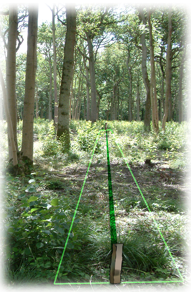
note peg at either end; central (dark) line which indicates aline of cord; pale outer line which indicates the plot area of 5om length
During the count (50×1 metre linear plot)
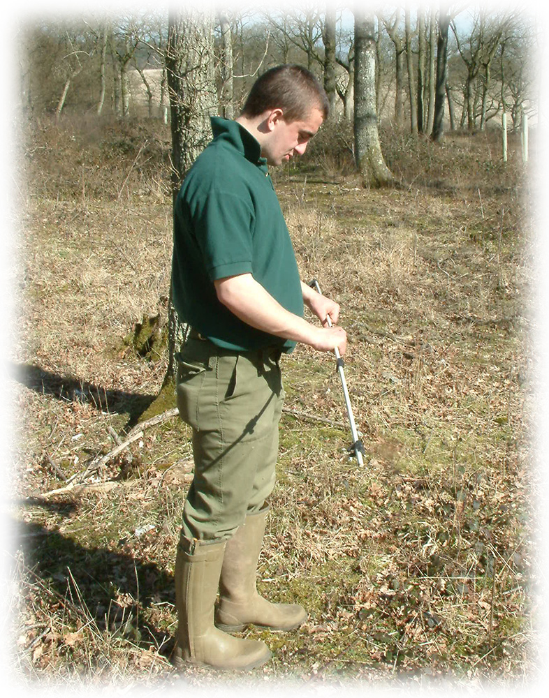
- At the first visit mark out permanent plots by placing a peg at either end and tying a cord between them. Position plots at random or choose a typical area of habitat, avoid crossing rides.
- For linear plots carry a rod the width of the plot (1 metre in this case) marked at the halfway point to help in judging whether pellet groups are in the plot, or outside and therefore not to be counted. It is not critical how groups that are on the edge of the plot are dealt with as long as rules are applied consistently e.g. a group could be “in” if any part of it is within 50cm of the survey line. Do not be tempted to include/exclude groups that do not meet your criteria, this will seriously bias results.
- Search carefully for pellet groups, counting those present ( not for use in this analysis but see additional interpretation below)
- Mark a sample of groups considered to be “fresh”. If these are still present on the return visit there will be some confidence that intermediate decomposition has not occurred
- Remove all other dung (use gloves) from the plot by casting them to one side.
- Remove the survey line but not the pegs
- Revisit the plots before new dung has time to decay, re-instate the survey line and count pellet groups accumulated on each plot, again using the rod as a guide
- Remove the survey line but not the pegs if intending to repeat in future
Calculating deer density
Defecation rates for individual species are necessary for calculating population densities. These are estimated as red (25 pellet groups per day), sika (25 pellet groups per day), fallow (20 pellet groups per day) and roe (20 pellet groups per day).
Example
Clearance counts were carried out in an area of deciduous woodland with sparse understory to estimate the density of roe deer. Pre-survey investigation of decay rate indicated a decay period of 6 months. 6 Plots totalling 600m2 were cleared in February. A total of 12 pellet groups (0.02 per m2) were counted in the plots 40 days later. Assuming a defecation rate of 20 pellet groups per day (and no decay between visits), the population density is estimated as:
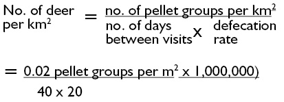
= 25 per km2
Results for each habitat in the area are obtained in a similar way. If the habitat is relatively uniform then repeat the survey in a number of areas.
It is possible to estimate deer numbers across the whole area by calculating how much of each habitat type is in the area, multiplying by the deer density in each then adding results for each habitat together.
Be aware of the potential error margins surrounding these calculations and therefore limitations in the value of the information generated as the sole basis for decision making.
Additional interpretation
When the plot is first visited it is worth noting:
- how many pellet groups were cleared. If the decay rate of pellets in the period preceding the count is known this figure can be used to calculate deer density using the FSC method.
- how many of groups were “fresh”, that is the surface of the pellets is intact, smooth, shiny and black. This helps to indicate that the area of the plot is currently in use by deer.
Reducing potential errors
There are a number of ways of avoiding sources of potential error:
- ensure that counters can distinguish deer dung from rabbits, hares etc, and where appropriate between deer species1 (for instance roe deer dung is rarely larger than 10mm in diameter)
- clearing pellet groups is usually more effective than marking
- stick rigidly to rules for include/ excluding groups in plots
- use same method on repeat counts or allow for changes e.g. to area surveyed
- as far as possible include as much of the deer range as possible in the count area, especially important with herding species.
Further Info
1 See the Deer Signs guide
Mayle, B.A., Peace, A.J. & Gill, R.M.A. (1999). How many deer? A field guide to estimating deer populations. Forestry Commission Fieldbook 18.
Swanson, G. Campbell, D. Armstrong, H. (2008) Estimating deer abundance in woodlands: the combination plot technique. Forestry Commission Bulletin 128.